RadxRate equations

Overview

RadxRate estimates the precipitation rate at each gate within a three-dimensional radar volume. RadxRate includes several equations for estimating precipitation rate, which can be tuned by the user for a specific environment and precipitation type. All coefficients for the equations are edited in the rate parameter file. This page will walk through these equations.

Polarimetric-based estimates

R(Z)

R(Z) equations are a simple way of estimating precipitation rates from the horizontal reflectivity factor (Z) and take the following form:

[math]\displaystyle{ R(Z)=aZ^b }[/math]

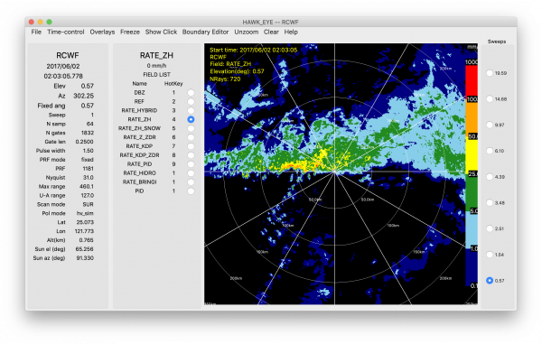
Many variations of this equation exist, depending on the precipitation type (e.g., convective or stratiform, tropical or mid-latitude). An example of the estimated precipitation from northern Taiwan using a tropical version of the equation ([math]\displaystyle{ R(Z)=0.027366Z^{0.69444} }[/math]) is shown in the image below. Since this example is from the lowest elevation angle, the echoes within ~150 km should all correspond to rain. R(Z) coefficients have been estimated for dry snow ([math]\displaystyle{ R(Z)=0.0365Z^{0.625} }[/math]), but aren't shown here given the warm environment near Taiwan.

R(Z, ZDR)

R(Z) relationships are known to be overly simplistic, as reflectivity depends on both hydrometeor size and concentration and single polarization only captures hydrometeor size in one dimension. Including ZDR helps mitigate the impact of big drops on Z. R(Z, ZDR) relationships take the form:

[math]\displaystyle{ R(Z,Z_{DR}) = aZ^bZ_{DR}^c }[/math]

An example of the estimated precipitation using coefficients from Berkowitz et al. (2013) is shown below ([math]\displaystyle{ R(Z,Z_{DR}) = 0.0067Z^{0.927}Z_{DR}^{-3.43} }[/math]).

R(KDP)

KDP has been used to estimate precipitation due to its relationship to the rain water content that slows down the propagating wave. Benefits of R(KDP) algorithms include insensitivity to radar calibration, attenuation, partial beam blockage, and ground clutter (Zrnić and Ryzhkov 1996), though care must be taken in the choice of filters used to calculate KDP and in Mie-scattering regimes. In RadxRate, R(KDP) takes the following form:

[math]\displaystyle{ R(K_{DP}) = sign(K_{DP})a\left|K_{DP}\right|^b }[/math]

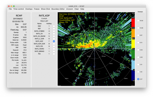
An example of the estimated precipitation using coefficients from Berkowitz et al. (2013) is shown below ([math]\displaystyle{ R(K_{DP}) = sign(K_{DP})44.0\left|K_{DP}\right|^{0.822} }[/math]). Note that R(KDP) output has more missing data than other algorithms.

R(KDP, ZDR)

Like R(Z, ZDR) algorithms, R(KDP, ZDR) algorithms combine the rain water content and particle size information that can be inferred from KDP and ZDR. In LROSE, these algorithms take the following form:

[math]\displaystyle{ R(K_{DP},Z_{DR}) = sign(K_{DP})a\left|K_{DP}\right|^bZ_{DR}^c }[/math]

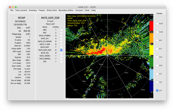
An example of the estimated precipitation using coefficients from Bringi and Chandrasekar (2001) and Brandes et al. (2002) is shown below ([math]\displaystyle{ R(K_{DP},Z_{DR}) = sign(K_{DP})90.8\left|K_{DP}\right|^{0.93}Z_{DR}^{-2.86} }[/math]). Note that R(KDP, ZDR) output has more missing data than other algorithms.

PID-based estimates

In addition to the aforementioned relationships that estimate precipitation rates directly from polarimetric variables, RadxRate includes relationships that prescribe different relationships based on the dominant hydrometeor type inferred from the polarimetric radar data. For example, these PID-based algorithms will use different equations for gates dominated by large raindrops and dry snow. All require the PID algorithm to be applied to the radar volume, which is done in an earlier step of RadxRate.

NCAR Hybrid

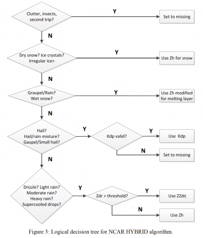
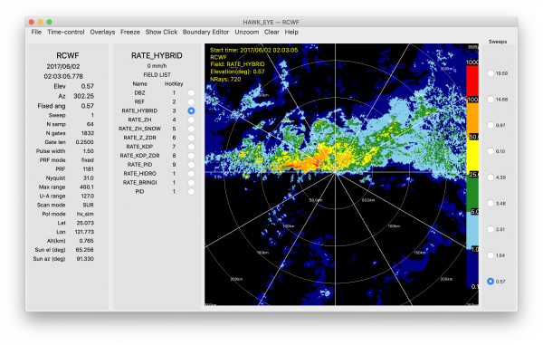
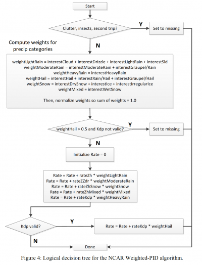
The NCAR Hybrid method applies some of the aforementioned precipitation rate equations to different PID categories. The method is described in the logical decision tree below (Dixon et al. 2015) and an example of the NCAR Hybrid method is also shown (right image).

NCAR Weighted-PID

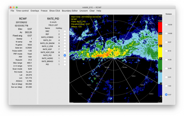
The NCAR Weighted-PID method applies some of the aforementioned precipitation rate equations to different PID categories, which are weighted by the interest values assigned by the PID algorithm. The method is described in the logical decision tree below (Dixon et al. 2015) and an example of the NCAR Weighted-PID method is also shown (right image).

CSU HIDRO

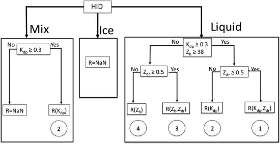
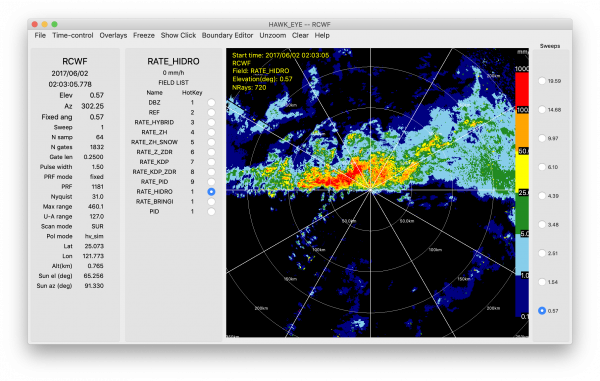
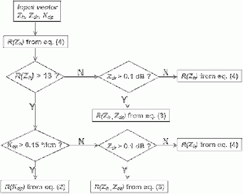
Like the NCAR Hybrid method, the CSU HIDRO method applies the aforementioned precipitation rate equations to different PID categories. The method is described in the logical decision tree below (Cifelli et al. 2011) and an example of the CSU HIDRO method is also shown (right image).

Bringi

Like the NCAR Hybrid method, the Bringi method applies the aforementioned precipitation rate equations to different PID categories. The method is described in the logical decision tree below (Bringi et al. 2009) and an example of the Bringi method is also shown (right image). We note that the equations mentioned in the linked citation were optimized for a C-band radar.

References

Berkowitz, D. S., J. A Schultz, S. Vasiloff, K.L. Elmore, C.D. Payne and J.B. Boettcher, 2013: Status of Dual Pol QPE in the WSR-88D Network. AMS 27th conference on hydrology, Austin, Texas, 2.2. Link

Brandes, E. A., G. Zhang, and J. Vivekanandan, 2002: Experiments in rainfall estimation with a polarimetric radar in a subtropical environment. J. Appl. Meteor., 41, 674–685. Link

Bringi, V. N., and V. Chandrasekar, 2001: Polarimetric Doppler Weather Radar. Principles and Applications. Cambridge University Press, 636 pp. Book

Bringi, V. N., Williams, C. R., Thurai, M., & May, P. T. (2009). Using Dual-Polarized Radar and Dual-Frequency Profiler for DSD Characterization: A Case Study from Darwin, Australia, Journal of Atmospheric and Oceanic Technology, 26(10), 2107-2122. Link

Cifelli, R., Chandrasekar, V., Lim, S., Kennedy, P. C., Wang, Y., & Rutledge, S. A. (2011). A New Dual-Polarization Radar Rainfall Algorithm: Application in Colorado Precipitation Events, Journal of Atmospheric and Oceanic Technology, 28(3), 352-364. Link

Dixon, M. J., J. W. Wilson, T. M. Weckwerth, D. Albo, and E. J. Thompson, 2015: A dual-polarization QPE method based on the NCAR particle ID algorithm: Description and preliminary results. 37th Conf. on Radar Meteorology, Norman, OK, Amer. Meteor. Soc., 9A.1. Link

Ryzhkov, A. V., Giangrande, S. E., & Schuur, T. J. (2005). Rainfall Estimation with a Polarimetric Prototype of WSR-88D, Journal of Applied Meteorology, 44(4), 502-515. Link

Zrnić, D. S., and A. Ryzhkov. 1996. Advantages of rain measurements using specific differential phase. J. Atmos. Oceanic Technol. 13:454–464. Link