Difference between revisions of "Csu radartools tutorial"
From Lrose Wiki
| (49 intermediate revisions by the same user not shown) | |||
| Line 1: | Line 1: | ||
| − | + | = '''Overview'''= | |
---- | ---- | ||
This tutorial will walk through the steps to read and convert a raw radar file, quality control the data (removing unwanted artifacts and echoes, unfold radial velocity and calculate Kdp), then grid the data, and finally process the gridded data to end up with hydrometeor identification, precipitation rates, and DSD information. This is generally focused on surface polarimetric X, C, or S-band radar. | This tutorial will walk through the steps to read and convert a raw radar file, quality control the data (removing unwanted artifacts and echoes, unfold radial velocity and calculate Kdp), then grid the data, and finally process the gridded data to end up with hydrometeor identification, precipitation rates, and DSD information. This is generally focused on surface polarimetric X, C, or S-band radar. | ||
| Line 9: | Line 9: | ||
* Despeckle and remove 2nd trip | * Despeckle and remove 2nd trip | ||
| − | + | Note: Every radar dataset is different -- these steps are for demonstration purposes only! | |
| + | |||
| + | = '''Modules available from GitHub'''= | ||
---- | ---- | ||
| Line 15: | Line 17: | ||
*https://github.com/CSU-Radarmet/CSU_RadarTools | *https://github.com/CSU-Radarmet/CSU_RadarTools | ||
| − | + | = '''Scientific Background'''= | |
---- | ---- | ||
| − | + | ===Kdp calculation=== | |
Hubbert, J., and V. N. Bringi. "An iterative filtering technique for the analysis of copolar differential phase and dual-frequency radar measurements." Journal of Atmospheric and Oceanic Technology 12.3 (1995): 643-648. | Hubbert, J., and V. N. Bringi. "An iterative filtering technique for the analysis of copolar differential phase and dual-frequency radar measurements." Journal of Atmospheric and Oceanic Technology 12.3 (1995): 643-648. | ||
| + | <br/> | ||
| + | |||
| + | ===Attenuation Correction=== | ||
| + | Carey, L. D., Rutledge, S. A., Ahijevych, D. A., & Keenan, T. D. (2000). Correcting propagation effects in C-band polarimetric radar observations of tropical convection using differential propagation phase. Journal of Applied Meteorology and Climatology, 39(9), 1405-1433. | ||
| + | <br/> | ||
| + | |||
| + | ===QC using standard deviation of the phase and Rho_hv=== | ||
| + | Ryzhkov, Alexander V., and Dusan S. Zrnic. "Polarimetric rainfall estimation in the presence of anomalous propagation." Journal of Atmospheric and Oceanic Technology 15, no. 6 (1998): 1320-1330. | ||
| + | <br/> | ||
| − | + | ='''Step-by-step Instructions'''= | |
---- | ---- | ||
The Example file is from the C-band polarimetric SEA-POL radar. The raw data are in sigmet native format.<br/> | The Example file is from the C-band polarimetric SEA-POL radar. The raw data are in sigmet native format.<br/> | ||
<br/> | <br/> | ||
| − | + | ||
| + | == Python Imports == | ||
| + | These are the imports needed for the code throughout this tutorial. | ||
| + | |||
import numpy as np | import numpy as np | ||
from copy import deepcopy | from copy import deepcopy | ||
import os | import os | ||
import pyart | import pyart | ||
| − | from | + | from csu_radartools import csu_kdp |
| − | from | + | from csu_radartools import csu_misc |
| + | import scipy.ndimage as ndi | ||
<br/> | <br/> | ||
| − | + | == Convert to CFRADIAL == | |
<br/> | <br/> | ||
Convert the data to cfradial data to be more easily transferable to other programs.<br/> | Convert the data to cfradial data to be more easily transferable to other programs.<br/> | ||
| Line 46: | Line 61: | ||
cfrad.20190917_071006.545_to_20190917_071353.149_SEAPOL_SUR.nc<br/> | cfrad.20190917_071006.545_to_20190917_071353.149_SEAPOL_SUR.nc<br/> | ||
<br/> | <br/> | ||
| + | We can read this into radar with pyart: | ||
| + | radar = pyart.io.read(f'{mydir}cfrad/cfrad.20190917_071006.545_to_20190917_071353.149_SEAPOL_SUR.nc') | ||
| + | |||
There are a lot of variables in this file, but the ones of interest are:<br/> | There are a lot of variables in this file, but the ones of interest are:<br/> | ||
| + | radar.fields.keys()<br/> | ||
DBZ: Reflectivity<br/> | DBZ: Reflectivity<br/> | ||
ZDR: Differential Reflectivity<br/> | ZDR: Differential Reflectivity<br/> | ||
| Line 56: | Line 75: | ||
</br> | </br> | ||
| − | + | == QC with CSU_Radartools and PyART == | |
Do some quality control using PyART and CSU_Radartools.</br> | Do some quality control using PyART and CSU_Radartools.</br> | ||
<br/> | <br/> | ||
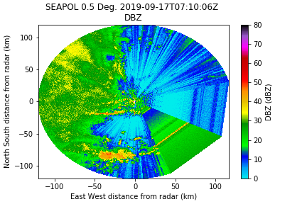
| + | Here is the original reflectivity field:<br/> | ||
| + | [[File:SEAPOL_example_origDZ.png|600px]] | ||
| + | |||
====Special handling for SEA-POL==== | ====Special handling for SEA-POL==== | ||
These are PECULIARS to the SEA-POL data. YMMV</br> | These are PECULIARS to the SEA-POL data. YMMV</br> | ||
| Line 72: | Line 94: | ||
radar.fields[f]['data'][j+1].mask = True | radar.fields[f]['data'][j+1].mask = True | ||
<br/> | <br/> | ||
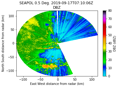
| + | The new reflectivity field is now masked over the wheelhouse:<br/> | ||
| + | [[File:SEAPOL_example_blankDZ.png|600px]] | ||
| + | |||
| + | |||
;The correlation coefficient is incorrect, but we can calculate it from UNKNONW_ID_82 field.<br/> | ;The correlation coefficient is incorrect, but we can calculate it from UNKNONW_ID_82 field.<br/> | ||
Now correct the UNKNOWN_ID_82 field to transform into the correlation coefficient (Again, this is only needed for this data).<br/><br/> | Now correct the UNKNOWN_ID_82 field to transform into the correlation coefficient (Again, this is only needed for this data).<br/><br/> | ||
| Line 79: | Line 105: | ||
radar.add_field_like('RHOHV','CC',ccorr) | radar.add_field_like('RHOHV','CC',ccorr) | ||
| − | + | ====Calculate Kdp==== | |
| − | This method uses the Hubbert and Bringi FIR filter method. We note that the window / gate spacing must be an even number or it will fail. it will also calculate the standard deviation of the phase which can be | + | This method uses the Hubbert and Bringi FIR filter method. We note that the window / gate spacing must be an even number or it will fail. it will also calculate the standard deviation of the phase which can be used to remove non-meteorological data.<br/><br/> |
| + | def extract_unmasked_data(radar, field, bad=-32768): | ||
| + | """Simplify getting unmasked radar fields from Py-ART""" | ||
| + | return radar.fields[field]['data'].filled(fill_value=bad)<br/> | ||
| + | dz_um = extract_unmasked_data(radar,'DBZ') | ||
| + | dp_um = extract_unmasked_data(radar, 'PHIDP')<br/> | ||
| + | Range needs to be supplied as a variable, and it needs to be the same shape as dzN, etc.<br/><br/> | ||
| + | rng2d, az2d = np.meshgrid(radar.range['data'], radar.azimuth['data']) | ||
| + | kdN, fdN, sdN = csu_kdp.calc_kdp_bringi(dp=dp_um, dz=dz_um, rng=rng2d/1000.0, thsd=12, gs=250.0, window=7, nfilter=2)<br/> | ||
| + | |||
| + | kdN is the specific differential phase, fdN is the filtered differential phase, and sdN is the standard deviation of the phase<br/> | ||
| + | Add this back into the radar structure.<br/><br/> | ||
| + | field_dict = {'data': kdN, | ||
| + | 'units': 'deg/km', | ||
| + | 'long_name': 'specific_differential_phase', | ||
| + | 'standard_name': 'Kdp', | ||
| + | '_FillValue': '-32768'} | ||
| + | radar.add_field('Kdp', field_dict, replace_existing=True) | ||
| + | |||
| + | ;Make sure the phase is between -180 and 180. | ||
| + | fdN[fdN<-180.0] += 360.0 | ||
| + | fdN[fdN>180.0] -= 360.0 | ||
| + | |||
| + | Save these to the radar object. | ||
| + | radar = radtools.add_field_to_radar_object(kdN, radar, field_name='KDP', units='deg/km', | ||
| + | long_name='CSU Specific Differential Phase', | ||
| + | standard_name='CSU Specific Differential Phase', | ||
| + | dz_field='DZQC') | ||
| + | radar = radtools.add_field_to_radar_object(fdN, radar, field_name='FDP', units='deg', | ||
| + | long_name='CSU Filtered Differential Phase', | ||
| + | standard_name='CSU Filtered Differential Phase', | ||
| + | dz_field='DZQC') | ||
| + | radar = radtools.add_field_to_radar_object(sdN, radar, field_name='SDP', units='deg', | ||
| + | long_name='CSU Standard Deviation of Differential Phase', | ||
| + | standard_name='CSU Standard Deviation of Differential Phase', | ||
| + | dz_field='DZQC') | ||
| + | |||
| + | ===Removing Non-meteorological Echoes=== | ||
| + | <br/> | ||
| + | ====Standard Deviation of Differential Phase==== | ||
| + | Sometimes the sdp goes nuts in high reflectivity regions, and pair this mask with relatively low dBZ regions. Here I am using a threshold of 10, but I usually do a sensitivity study to figure out a good value, typically ranging from 10 to 25. However, remember that things like hail can have high sdN. | ||
| + | sdp_mask = csu_misc.differential_phase_filter(sdN, thresh_sdp=13) | ||
| + | sdp_mask = np.logical_and(sdp_mask, radar.fields['DBZ']['data'] <= 10)<br/> | ||
| + | |||
| + | old_var_mask = deepcopy(radar.fields['DBZ']['data'].mask) | ||
| + | new_var_mask = np.logical_or(old_var_mask, sdp_mask) | ||
| + | radar.fields['DBZ']['data'].mask = new_var_mask | ||
| + | <br/> | ||
| + | [[File:SEAPOL_example_sdpDZ.png|600px]] | ||
| + | <br/> | ||
| + | Well that didn't get us vary far (this is not unexpected given the RF interference with this particular dataset). But we have other tools at our disposal, and this is usually paired with another filter like rho_hv or SQI. | ||
| + | |||
| + | ====SQI and/ or Rho_HV==== | ||
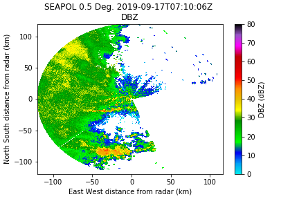
| + | Here I'm using SQI because it's available in the Sigmet data. We have found that 0.35 is an ok threshold for now. <br/> | ||
| + | sq_mask = radar.fields['SQI']['data'] < 0.35] | ||
| + | <br/> | ||
| + | [[File:SEAPOL_example_sqDZ.png|600px]] | ||
| + | <br/> | ||
| + | And for the heck of it, Rho_hv threshold of 0.8 for that extra little bit. | ||
| + | rho_mask = ccorr < 0.8 | ||
| + | |||
| + | Much better, but now we need a despeckler to pick up those random points. | ||
| + | |||
| + | ====Despeckler==== | ||
| + | We found that 4 gates works pretty well for this data. (remember that dz_um is the unmasked reflectivity that has the above corrections already applied).<br/> | ||
| + | |||
| + | mask_ds = csu_misc.despeckle(dz_um, ngates=4) | ||
| + | |||
| + | <br/> | ||
| + | [[File:SEAPOL_example_despeckDZ.png|600px]] | ||
| + | <br/> | ||
| + | Looking pretty good! | ||
| + | |||
| + | ====Insect Filter==== | ||
| + | Occasionally you will need to remove insects. This typically has high Zdr and moderate reflectivity. There is an insect_filter built into CSU_Radartools.<br/> | ||
| + | Note: This image does not have any insects so there is no change when applying this field, but here is how one does that. | ||
| + | |||
| + | insect_mask = csu_misc.insect_filter(dz_um, zdr_um, | ||
| + | dz_range=[[-100, 10], [10, 15], [15, 20], [20, 25], [25, 30], [30, 35]], | ||
| + | dr_thresh=[1, 1.3, 1.7, 2.1, 2.5, 2.8]) | ||
| + | |||
| + | ====Second Trip==== | ||
| + | Second trip can be hard to blanket-remove with any one variable, unless you have Ldr, in which case 2nd trip often shows up as positive values. The following methodology was developed by Dr. B. Fuchs and was found to work well on the SEA-POL data, using a smoothed SQI field. As always, be sure to use with caution on other datasets. | ||
| + | sm_g_rad = 5 | ||
| + | sqi_smooth = ndi.gaussian_filter(radar.fields['SQI']['data'], (sm_g_rad, sm_g_rad), mode='nearest') | ||
| + | second_trip_flag = np.ma.getdata((sqi_smooth <= 0.12)) | ||
| + | |||
| + | As with the insects, this is example does not have 2nd trip, and therefore this filter does not do anything. | ||
| + | |||
| + | |||
| + | ==Attenuation Correction== | ||
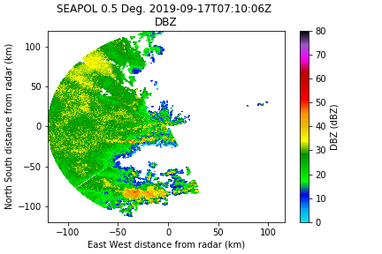
| + | This methodology is based on Carey et al. 2000.<br/> | ||
| + | Basically it calculates (or uses a default) coefficient in the A= a Kdp^b equation.<br/> | ||
| + | |||
| + | gate_heights = deepcopy(radar.get_gate_x_y_z(0)[-1]/1000.0) | ||
| + | for ins in range(1, radar.nsweeps): | ||
| + | gate_heights = np.concatenate((gate_heights, radar.get_gate_x_y_z(ins)[-1]/1000.0)) # want it in km | ||
| + | |||
| + | ;This is an experimental piece of CSU_Radartools and has not been implemented on the main branch. | ||
| + | zcorr, satt, zaa = csu_atten_corr.calc_atten(radar.fields['DBZ']['data'], | ||
| + | radar.fields['DP']['data'], | ||
| + | kd=radar.fields['KDP']['data'], | ||
| + | height=gate_heights, a_default=-0.15, deva=0.10, | ||
| + | bad=np.nan, force_default=False, phase_diff_calc=True, | ||
| + | min_pts=150) | ||
| + | {|class="wikitable" | ||
| + | !Original | ||
| + | !Corrected | ||
| + | |- | ||
| + | |[[File:SEAPOL_example_despeckDZ.png|600px]] | ||
| + | |[[File:SEAPOL_example_attenDZ.png|600px]] | ||
| + | |} | ||
| + | |||
| + | |||
| + | ;And to add in the differential reflectivity correction, we can specify diff_atten = True to use the correct coefficients. | ||
| + | |||
| + | zdrcorr, sadptt, zdpa = csu_atten_corr.calc_atten(radar.fields['ZDR']['data'], | ||
| + | radar.fields['DP']['data'], | ||
| + | kd=radar.fields['KDP']['data'], | ||
| + | height=gate_heights, a_default=-0.15, deva=0.10, | ||
| + | bad=np.nan, force_default=False, phase_diff_calc=True, | ||
| + | min_pts=150,diff_atten = True) | ||
| + | |||
| + | {|class="wikitable" | ||
| + | !Original | ||
| + | !Corrected | ||
| + | |- | ||
| + | |[[File:SEAPOL_example_ZDR.png|600px]] | ||
| + | |[[File:SEAPOL_example_attenDR.png|600px]] | ||
| + | |} | ||
| + | |||
| + | ==Unfolding Radial Velocity== | ||
| + | In PyART, there are several ways to automatically unfold the radial velocity field around the Nyquist. They all have strengths and weaknesses, and I usually try them all to see what works best on a given dataset. It happens that for this one, a simple unwrapping dealias works pretty well.<br/> | ||
| + | |||
| + | *pyart.correct.dealias_fourdd | ||
| + | *pyart.dealias_region_based | ||
| + | *pyart.correct.dealias_unwrap_phase | ||
| + | <br/> | ||
| + | NOTE: SEA-POL Nyquist is 15.9 m/s for this scan. | ||
| + | corrected_velocity = pyart.correct.dealias_unwrap_phase(radar, vel_field='VEL', corr_vel_field='CV') | ||
| + | <br/> | ||
| + | corr_vel_region = pyart.correct.dealias_region_based(radar,vel_field='VEL',nyquist_vel=15.9) | ||
| + | <br/> | ||
| + | |||
| + | {|class="wikitable" | ||
| + | !Original | ||
| + | !Unwrap Phase | ||
| + | !Region Based | ||
| + | |- | ||
| + | |[[File:SEAPOL_example_VEL.png|600px]] | ||
| + | |[[File:SEAPOL_example_unwrapCV.png|600px]] | ||
| + | |[[File:SEAPOL_example_regionCV.png|600px]] | ||
| + | |||
| + | |} | ||
| + | We can see that there are some errors in this correction method. Sometimes this method works better with unfiltered data, and I could probably play with the parameters a bit to clean it up, but the phase-based method worked pretty good so we will go with that. | ||
| + | ==Grid data with Radx2Grid== | ||
| + | Once we are happy with the changes we've made, we can write out a file with pyart. | ||
| + | cfqcfile = f'{mydir}SEA20190917_071005_qced.cfrad.nc' | ||
| + | pyart.io.write_cfradial(cfqcfile,radar) | ||
| − | + | And we can setup the things for calling Radx2Grid from the command line. | |
| + | params_file = Radx2Grid.seapol.piston.cart | ||
| + | outpath = f'{mydir}/grid' | ||
| + | radgrid_command = f'Radx2Grid -params {params_file} -f {cfqcfile} -outdir {outpath}' | ||
| + | os.system(radgrid_command) | ||
Latest revision as of 16:31, 26 August 2021
Contents
Overview
This tutorial will walk through the steps to read and convert a raw radar file, quality control the data (removing unwanted artifacts and echoes, unfold radial velocity and calculate Kdp), then grid the data, and finally process the gridded data to end up with hydrometeor identification, precipitation rates, and DSD information. This is generally focused on surface polarimetric X, C, or S-band radar. We will apply a series of corrections
- Unfold radial velocity
- Calculate Kdp
- Apply thresholds to remove non-meteorological data
- Calculate the attenuation and differential attenuation
- Despeckle and remove 2nd trip
Note: Every radar dataset is different -- these steps are for demonstration purposes only!
Modules available from GitHub
Scientific Background
Kdp calculation
Hubbert, J., and V. N. Bringi. "An iterative filtering technique for the analysis of copolar differential phase and dual-frequency radar measurements." Journal of Atmospheric and Oceanic Technology 12.3 (1995): 643-648.
Attenuation Correction
Carey, L. D., Rutledge, S. A., Ahijevych, D. A., & Keenan, T. D. (2000). Correcting propagation effects in C-band polarimetric radar observations of tropical convection using differential propagation phase. Journal of Applied Meteorology and Climatology, 39(9), 1405-1433.
QC using standard deviation of the phase and Rho_hv
Ryzhkov, Alexander V., and Dusan S. Zrnic. "Polarimetric rainfall estimation in the presence of anomalous propagation." Journal of Atmospheric and Oceanic Technology 15, no. 6 (1998): 1320-1330.
Step-by-step Instructions
The Example file is from the C-band polarimetric SEA-POL radar. The raw data are in sigmet native format.
Python Imports
These are the imports needed for the code throughout this tutorial.
 import numpy as np
 from copy import deepcopy
 import os
 import pyart
 from csu_radartools import csu_kdp
 from csu_radartools import csu_misc
 import scipy.ndimage as ndi
Convert to CFRADIAL
Convert the data to cfradial data to be more easily transferable to other programs.
We can do this using RadxConvert from a command line, but we can also do it from python with the os command.
 mydir = '/Users/bdolan/scratch/LROSE/SEA-POL/ppi/'
 os.system(f'RadxConvert -f {mydir}SEA20190917_071005 -outdir {mydir}cfrad')
This will put the output in a directory for the date in directory 'cfrad'.
Now we have a file called:
cfrad.20190917_071006.545_to_20190917_071353.149_SEAPOL_SUR.nc
We can read this into radar with pyart:
radar = pyart.io.read(f'{mydir}cfrad/cfrad.20190917_071006.545_to_20190917_071353.149_SEAPOL_SUR.nc')
There are a lot of variables in this file, but the ones of interest are:
radar.fields.keys()
DBZ: Reflectivity
ZDR: Differential Reflectivity
UNKNOWN_ID_82: Correlation Coefficient
VEL: Radial velocity
SQI: Signal Quality Index
PHIDP: Differential phase
SNR: Signal to noise ratio
QC with CSU_Radartools and PyART
Do some quality control using PyART and CSU_Radartools.
Here is the original reflectivity field:
Special handling for SEA-POL
These are PECULIARS to the SEA-POL data. YMMV
- Blanked sector over the wheelhouse
We will look for large blocks of azimuthal jumps to mask them. Get the difference between each azimuth and look for jumps larger than 30º. If so, mask the data so it plots correctly.
az_diff = np.diff(radar.azimuth['data'])
jumps = np.where(np.abs(az_diff) >= 30.0)[0]
if len(jumps):
  for f in radar.fields.keys():
     for j in jumps:
        radar.fields[f]['data'][j].mask = True
        radar.fields[f]['data'][j+1].mask = True
The new reflectivity field is now masked over the wheelhouse:
- The correlation coefficient is incorrect, but we can calculate it from UNKNONW_ID_82 field.
Now correct the UNKNOWN_ID_82 field to transform into the correlation coefficient (Again, this is only needed for this data).
 ccorr = deepcopy(radar.fields['UNKNOWN_ID_82']['data'])
 ccorr[ccorr<0] += 65535
 ccorr = (ccorr-1)/65533.0
 radar.add_field_like('RHOHV','CC',ccorr)
Calculate Kdp
This method uses the Hubbert and Bringi FIR filter method. We note that the window / gate spacing must be an even number or it will fail. it will also calculate the standard deviation of the phase which can be used to remove non-meteorological data.
 def extract_unmasked_data(radar, field, bad=-32768):
   """Simplify getting unmasked radar fields from Py-ART"""
   return radar.fields[field]['data'].filled(fill_value=bad)

 dz_um = extract_unmasked_data(radar,'DBZ')
 dp_um = extract_unmasked_data(radar, 'PHIDP')
Range needs to be supplied as a variable, and it needs to be the same shape as dzN, etc.
 rng2d, az2d = np.meshgrid(radar.range['data'], radar.azimuth['data'])
 kdN, fdN, sdN = csu_kdp.calc_kdp_bringi(dp=dp_um, dz=dz_um, rng=rng2d/1000.0, thsd=12, gs=250.0, window=7, nfilter=2)
kdN is the specific differential phase, fdN is the filtered differential phase, and sdN is the standard deviation of the phase
Add this back into the radar structure.
 field_dict = {'data': kdN,
               'units': 'deg/km',
               'long_name': 'specific_differential_phase',
               'standard_name': 'Kdp',
               '_FillValue': '-32768'}
 radar.add_field('Kdp', field_dict, replace_existing=True)
- Make sure the phase is between -180 and 180.
  fdN[fdN<-180.0] += 360.0
  fdN[fdN>180.0] -= 360.0
Save these to the radar object.
  radar = radtools.add_field_to_radar_object(kdN, radar, field_name='KDP', units='deg/km',
                                      long_name='CSU Specific Differential Phase',
                                      standard_name='CSU Specific Differential Phase',
                                      dz_field='DZQC')
  radar = radtools.add_field_to_radar_object(fdN, radar, field_name='FDP', units='deg',
                                      long_name='CSU Filtered Differential Phase',
                                      standard_name='CSU Filtered Differential Phase',
                                      dz_field='DZQC')
  radar = radtools.add_field_to_radar_object(sdN, radar, field_name='SDP', units='deg',
                                      long_name='CSU Standard Deviation of Differential Phase',
                                      standard_name='CSU Standard Deviation of Differential Phase',
                                      dz_field='DZQC')
Removing Non-meteorological Echoes
Standard Deviation of Differential Phase
Sometimes the sdp goes nuts in high reflectivity regions, and pair this mask with relatively low dBZ regions. Here I am using a threshold of 10, but I usually do a sensitivity study to figure out a good value, typically ranging from 10 to 25. However, remember that things like hail can have high sdN.
  sdp_mask = csu_misc.differential_phase_filter(sdN, thresh_sdp=13)
  sdp_mask = np.logical_and(sdp_mask, radar.fields['DBZ']['data'] <= 10)
  old_var_mask = deepcopy(radar.fields['DBZ']['data'].mask)
  new_var_mask = np.logical_or(old_var_mask, sdp_mask)
  radar.fields['DBZ']['data'].mask = new_var_mask

Well that didn't get us vary far (this is not unexpected given the RF interference with this particular dataset). But we have other tools at our disposal, and this is usually paired with another filter like rho_hv or SQI.
SQI and/ or Rho_HV
Here I'm using SQI because it's available in the Sigmet data. We have found that 0.35 is an ok threshold for now.
sq_mask = radar.fields['SQI']['data'] < 0.35]
And for the heck of it, Rho_hv threshold of 0.8 for that extra little bit.
rho_mask = ccorr < 0.8
Much better, but now we need a despeckler to pick up those random points.
Despeckler
We found that 4 gates works pretty well for this data. (remember that dz_um is the unmasked reflectivity that has the above corrections already applied).
mask_ds = csu_misc.despeckle(dz_um, ngates=4)
Insect Filter
Occasionally you will need to remove insects. This typically has high Zdr and moderate reflectivity. There is an insect_filter built into CSU_Radartools.
Note: This image does not have any insects so there is no change when applying this field, but here is how one does that.
  insect_mask = csu_misc.insect_filter(dz_um, zdr_um,
    dz_range=[[-100, 10], [10, 15], [15, 20], [20, 25], [25, 30], [30, 35]],
    dr_thresh=[1, 1.3, 1.7, 2.1, 2.5, 2.8])
Second Trip
Second trip can be hard to blanket-remove with any one variable, unless you have Ldr, in which case 2nd trip often shows up as positive values. The following methodology was developed by Dr. B. Fuchs and was found to work well on the SEA-POL data, using a smoothed SQI field. As always, be sure to use with caution on other datasets.
   sm_g_rad = 5
   sqi_smooth = ndi.gaussian_filter(radar.fields['SQI']['data'], (sm_g_rad, sm_g_rad), mode='nearest')
   second_trip_flag = np.ma.getdata((sqi_smooth <= 0.12))
As with the insects, this is example does not have 2nd trip, and therefore this filter does not do anything.
Attenuation Correction
This methodology is based on Carey et al. 2000.
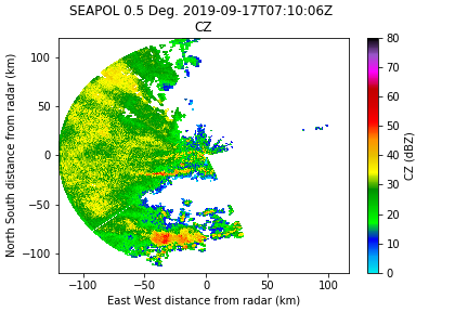
Basically it calculates (or uses a default) coefficient in the A= a Kdp^b equation.
  gate_heights = deepcopy(radar.get_gate_x_y_z(0)[-1]/1000.0)
  for ins in range(1, radar.nsweeps):
     gate_heights = np.concatenate((gate_heights, radar.get_gate_x_y_z(ins)[-1]/1000.0)) # want it in km
- This is an experimental piece of CSU_Radartools and has not been implemented on the main branch.
  zcorr, satt, zaa = csu_atten_corr.calc_atten(radar.fields['DBZ']['data'],
             radar.fields['DP']['data'],
             kd=radar.fields['KDP']['data'],
             height=gate_heights, a_default=-0.15, deva=0.10,
             bad=np.nan, force_default=False, phase_diff_calc=True,
             min_pts=150)
| Original | Corrected |
|---|---|
|
|
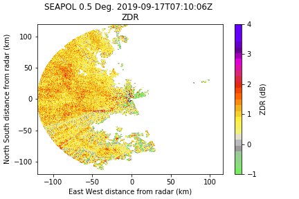
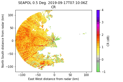
- And to add in the differential reflectivity correction, we can specify diff_atten = True to use the correct coefficients.
  zdrcorr, sadptt, zdpa = csu_atten_corr.calc_atten(radar.fields['ZDR']['data'],
             radar.fields['DP']['data'],
             kd=radar.fields['KDP']['data'],
             height=gate_heights, a_default=-0.15, deva=0.10,
             bad=np.nan, force_default=False, phase_diff_calc=True,
             min_pts=150,diff_atten = True)
| Original | Corrected |
|---|---|
|
|
Unfolding Radial Velocity
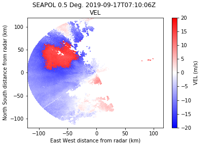
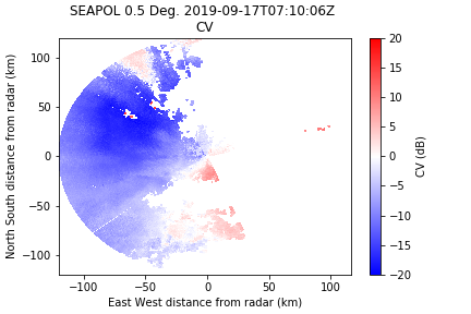
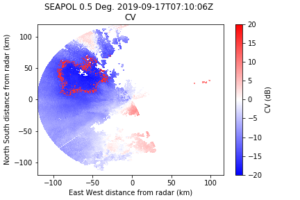
In PyART, there are several ways to automatically unfold the radial velocity field around the Nyquist. They all have strengths and weaknesses, and I usually try them all to see what works best on a given dataset. It happens that for this one, a simple unwrapping dealias works pretty well.
- pyart.correct.dealias_fourdd
- pyart.dealias_region_based
- pyart.correct.dealias_unwrap_phase
NOTE: SEA-POL Nyquist is 15.9 m/s for this scan.
corrected_velocity = pyart.correct.dealias_unwrap_phase(radar, vel_field='VEL', corr_vel_field='CV')
corr_vel_region = pyart.correct.dealias_region_based(radar,vel_field='VEL',nyquist_vel=15.9)
| Original | Unwrap Phase | Region Based |
|---|---|---|
|
|
|
We can see that there are some errors in this correction method. Sometimes this method works better with unfiltered data, and I could probably play with the parameters a bit to clean it up, but the phase-based method worked pretty good so we will go with that.
Grid data with Radx2Grid
Once we are happy with the changes we've made, we can write out a file with pyart.
   cfqcfile = f'{mydir}SEA20190917_071005_qced.cfrad.nc'
   pyart.io.write_cfradial(cfqcfile,radar)
And we can setup the things for calling Radx2Grid from the command line.
   params_file = Radx2Grid.seapol.piston.cart
   outpath = f'{mydir}/grid'
   radgrid_command = f'Radx2Grid -params {params_file} -f {cfqcfile} -outdir {outpath}'
   os.system(radgrid_command)